Lines as Boolean Classifiers
Introduction
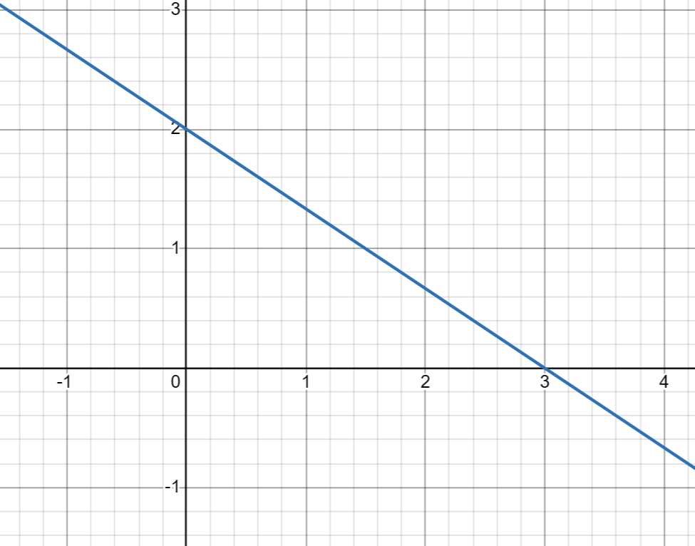
How can we find the equation of this line?
We know that two points on the line are
\[(0,2)\]and
\[(3,0).\]The standard equation of a line in two dimensions is
\[x_2 = m x_1 + c\]where
- $m$ is the slope of the line,
- $c$ is the intercept, which determines where the line crosses the $x_2$-axis.
Sometimes this is written as
\[y = mx + c.\]However, throughout this tutorial we will use machine learning notation where each sample consists of features $x_1$ and $x_2$.
Since the point
\[(0,2)\]lies on the line, we immediately know that
\[c = 2.\]The slope can be computed from the two points:
\[m = \frac{\Delta x_2}{\Delta x_1} = \frac{0-2}{3-0} = -\frac{2}{3}.\]Therefore,
\[x_2 = -\frac{2}{3}x_1 + 2.\]This is the equation of our line.
Vector Form of a Line
In machine learning, lines are usually written in a different form:
\[a x_1 + b x_2 + c = 0.\]Starting from
\[x_2 = -\frac{2}{3}x_1 + 2,\]we move everything to one side:
\[-\frac{2}{3}x_1 - x_2 + 2 = 0.\]The coefficients of the variables become the learnable parameters of our model.
We therefore write
\[w_1x_1 + w_2x_2 + b = 0.\]For our particular line:
\[w_1 = -\frac{2}{3}, \qquad w_2 = -1, \qquad b = 2.\]Vector Notation
Instead of writing each feature separately, we collect them into vectors:
\[\mathbf{w} = [w_1,w_2]\]and
\[\mathbf{x} = [x_1,x_2].\]The line can then be written compactly as
\[\mathbf{w}\cdot\mathbf{x}+b=0.\]Here $\mathbf{w}\cdot\mathbf{x}$ denotes the dot product.
This notation is used extensively throughout machine learning because it scales naturally to higher dimensions.
The Weight Vector
An important geometric fact is:
The weight vector is always perpendicular (orthogonal) to the line.
For our example,
\[\mathbf{w} = \left[ -\frac{2}{3}, -1 \right].\]
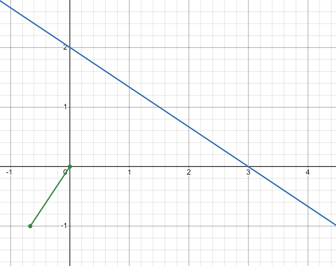
This vector points down and to the left.
To make the geometry easier to visualize, we can multiply the entire vector by $-1$:
\[\left[ \frac{2}{3}, 1 \right].\]
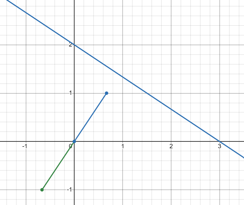
Multiplying by $-1$ does not change the normal direction. It only flips which way the arrow points.
The line itself remains exactly the same.
Finding the Closest Point on the Line
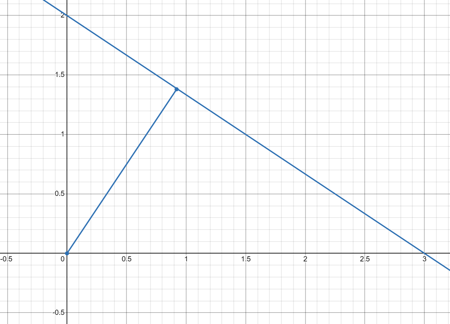
The normal vector starts at the origin and intersects the line at exactly one point.
Suppose this touching point has the form
\[t \left[ \frac{2}{3}, 1 \right] = \left[ \frac{2}{3}t, t \right].\]Because this point lies on the line, it must satisfy
\[-\frac{2}{3}x_1 - x_2 + 2 = 0.\]Substituting
\[x_1=\frac{2}{3}t, \qquad x_2=t\]gives
\[-\frac{2}{3} \left( \frac{2}{3}t \right) - t + 2 = 0.\]Simplifying:
\[-\frac{4}{9}t - t + 2 = 0\] \[-\frac{13}{9}t + 2 = 0\] \[t = \frac{18}{13}.\]Therefore the touching point is
\[\left[ \frac{2}{3}\cdot\frac{18}{13}, \frac{18}{13} \right] = \left[ \frac{12}{13}, \frac{18}{13} \right] \approx [0.92,1.38].\]
The Infinite Family of Normal Vectors
A normal vector is defined entirely by its direction.
Any nonzero scalar multiple of a normal vector is still a normal vector.
For example:
- $[2,3]$
- $[\frac{2}{3},1]$
- $[-\frac{2}{3},-1]$
- $[200,300]$
All of these vectors lie on the same normal line and are perpendicular to the separator.
The length of the vector does not matter.
Only its direction matters.
Turning a Line into a Classifier
So far, our line has been purely geometric.
Now we want to use it as a classifier.
The equation
\[\mathbf{w}\cdot\mathbf{x}+b=0\]divides the plane into two regions.
Points on one side satisfy
\[\mathbf{w}\cdot\mathbf{x}+b > 0,\]while points on the other side satisfy
\[\mathbf{w}\cdot\mathbf{x}+b < 0.\]This allows us to define a binary classification rule:
\[h(\mathbf{x}) = \begin{cases} 1 & \text{if } \mathbf{w}\cdot\mathbf{x}+b > 0\\ 0 & \text{if } \mathbf{w}\cdot\mathbf{x}+b < 0 \end{cases}\]The line itself is the decision boundary because it corresponds to
\[\mathbf{w}\cdot\mathbf{x}+b=0.\]Testing Some Points
Using our line
\[-\frac{2}{3}x_1 - x_2 +2 =0,\]consider the point
\[(1,1).\]Substituting gives
\[-\frac{2}{3}(1)-1+2 = \frac{1}{3} > 0.\]Therefore this point lies on the positive side of the separator.
Now consider
\[(2,2).\]Substituting gives
\[-\frac{2}{3}(2)-2+2 = -\frac{4}{3} < 0.\]Therefore this point lies on the negative side of the separator.
Why the Weight Vector Matters
The weight vector is perpendicular to the decision boundary.
More importantly, it points toward the region where
\[\mathbf{w}\cdot\mathbf{x}+b\]becomes increasingly positive.
This means the weight vector acts as a directional reference that determines which side of the separator is considered positive.
Changing the sign of every weight flips this direction and swaps the interpretation of the two regions.
The decision boundary itself remains unchanged.
Learning the Separator from Data
So far, we manually chose
\[\mathbf{w} = \left[ -\frac{2}{3}, -1 \right]\]and
\[b=2.\]In a real machine learning problem, we are not given the correct separator.
Instead, we are given a collection of feature vectors
\[\mathbf{x}_i\]together with labels
\[y_i \in \{0,1\}.\]The goal of training is to automatically discover values for $\mathbf{w}$ and $b$ that correctly separate the classes.
Initially, most learning algorithms start with random values.
As a result, the line
\[\mathbf{w}\cdot\mathbf{x}+b=0\]usually points in a poor direction and misclassifies many training samples.
The task of learning is therefore to gradually rotate and shift the separator until it better aligns with the data.
What Does a Mistake Look Like?
Recall our classification rule:
\[\mathbf{w}\cdot\mathbf{x}+b > 0 \quad\Rightarrow\quad \text{Positive Class}\] \[\mathbf{w}\cdot\mathbf{x}+b < 0 \quad\Rightarrow\quad \text{Negative Class}.\]Suppose a sample has label
\[y_i = 1.\]If evaluating the line equation produces
\[\mathbf{w}\cdot\mathbf{x}_i+b < 0,\]then the sample lies on the wrong side of the separator.
Likewise, if
\[y_i = 0\]but
\[\mathbf{w}\cdot\mathbf{x}_i+b > 0,\]then a negative sample has been incorrectly classified as positive.
These mistakes provide the information needed to improve the separator.
The Perceptron Learning Rule
One of the earliest learning algorithms is the Perceptron.
Whenever a sample is misclassified, the weights are adjusted according to
\[w_j^{(t+1)} = w_j^{(t)} + \alpha \Big( y_i - h_{\mathbf{w}}(\mathbf{x}_i) \Big) x_j^{(i)}\]where
- $\alpha$ is the learning rate,
- $y_i$ is the true label,
- $h_{\mathbf{w}}(\mathbf{x}_i)$ is the prediction.
If the prediction is already correct, no update occurs.
Geometric Interpretation of Learning
The update rule has a simple geometric interpretation.
When a positive sample is misclassified, the algorithm adjusts the weight vector so that the positive region expands toward that sample.
When a negative sample is misclassified, the algorithm adjusts the weight vector in the opposite direction.
Because the separator is defined by
\[\mathbf{w}\cdot\mathbf{x}+b=0,\]changing the weights rotates the separator, while changing the bias shifts it.
Training therefore consists of repeatedly rotating and shifting the line until it agrees with the labels observed in the data.
The Big Picture
A linear classifier is ultimately just a line together with a chosen direction.
The equation
\[\mathbf{w}\cdot\mathbf{x}+b=0\]defines the decision boundary.
The weight vector $\mathbf{w}$ determines which side of that boundary is considered positive.
Learning is the process of automatically adjusting $\mathbf{w}$ and $b$ until the boundary and its orientation correctly separate the training data.